
Complex math always scares me. Mathematical functions written on the paper never made any sense to me. But i used to find it interesting to plot these functions and see the shapes they produce.But plotting them with pencil and paper was painful and took lot of time. Later after I learnt some elementary programming in C, I generated datasets with simple programs and tried using putpixel(x,y) like functions, to plot them on screen. Even that wasn't easy and dint get smooth curves.
Now i am trying to do the same exercise using a powerful tool of the GNU tool chain - Gnuplot. Its available free with almost all Linux distros or can be downloaded for free from here. Debian users can use
sudo apt-get install gnuplot
Getting started with gnuplot
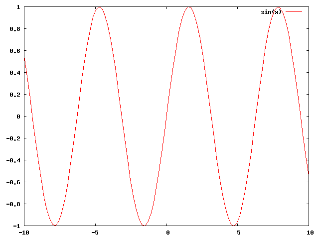
gnuplot is extremely user/programmer friendly. Just type 'gnuplot' to get the gnuplot shell. I wanted to see my favorite Sine wave first.
gnuplot> plot sin(x) Thats it and i got my first function plotted on gnuplot. It cant get anymore simple..!
Saving output to file
Next I wanted to save the graph as an image file.
gnuplot> set terminal png gnuplot> set output "sine.png" gnuplot> replot
Now the output is dumped into "sine.png" in the current directory.
'replot' simply repeats the last 'plot' call.
Plotting multiple functions in the same graph
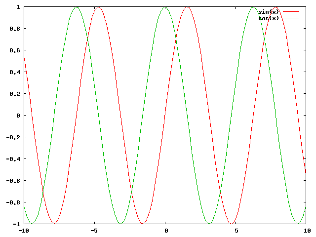
Intuitive ways work perfectly on gnuplot. To plot sine and cos waves on the same graph : gnuplot> plot sin(x),cos(x) OR gnuplot> plot sin(x) gnuplot> replot cos(x)
replot adds its arguments to the previous plot's argument list and then calls plot again.
Plotting parametric equations
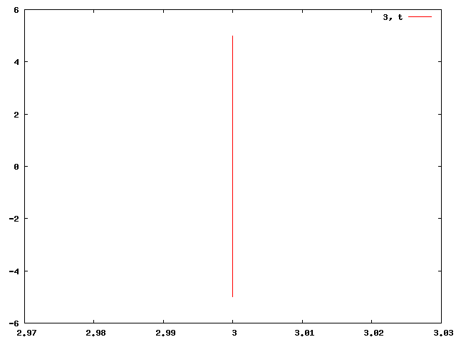
- Line
x = constant y = t
gnuplot> set parametric gnuplot> plot 3,t
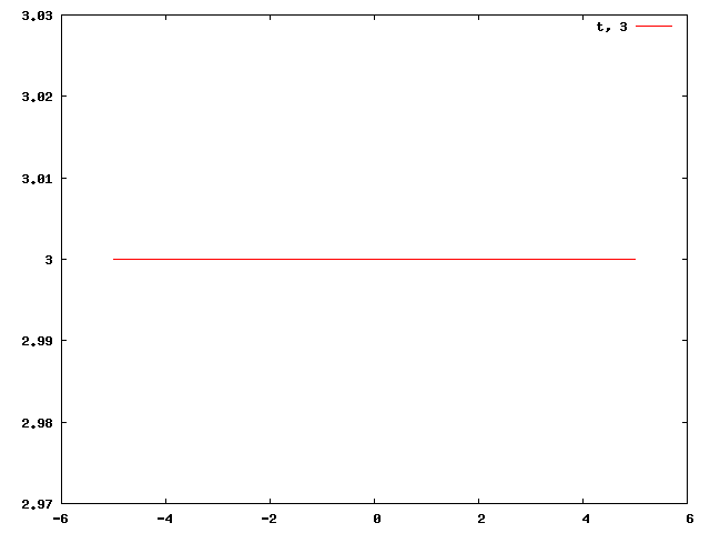
gnuplot> plot t,3
- Square
Basically 2 vertical and 2 horizontal striaght lines.
gnuplot> set parametric gnuplot> set xrange[-2:8] gnuplot> set yrange[-2:8] gnuplot> set trange[0:4] gnuplot> plot 0,t gnuplot> replot 4,t gnuplot> replot t,0 gnuplot> replot t,4
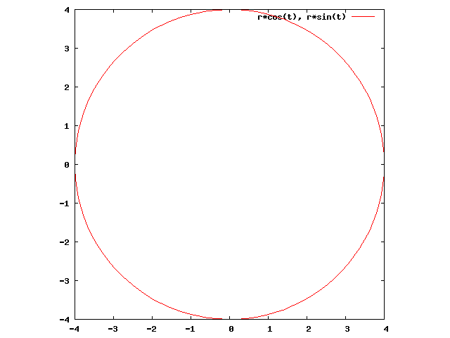
- Circle Circle of radius r and centered at (a,b) :
x = r * Cos(t) + a y = r * Sin(t) + b
gnuplot> set parametric gnuplot> set angle degree gnuplot> set trange [0:360] gnuplot> set size square gnuplot> r = 4 gnuplot> plot rcos(t), rsin(t)
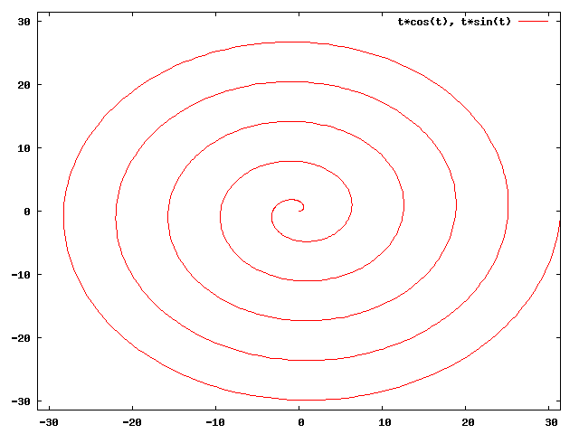
- Spiral In the circle's equation, instead of keeping radius constant, if we make it a function of t, we get a spiral (when r(t) = t)
x = r(t) * Cos(t) + a y = r(t) * Sin(t) + br(t) = t
gnuplot> set parametric gnuplot> set trange [0:10pi] gnuplot> set xrange[-10pi:10pi] gnuplot> set yrange[-10pi:10pi] gnuplot> set samples 1000 gnuplot> plot tcos(t), t*sin(t)
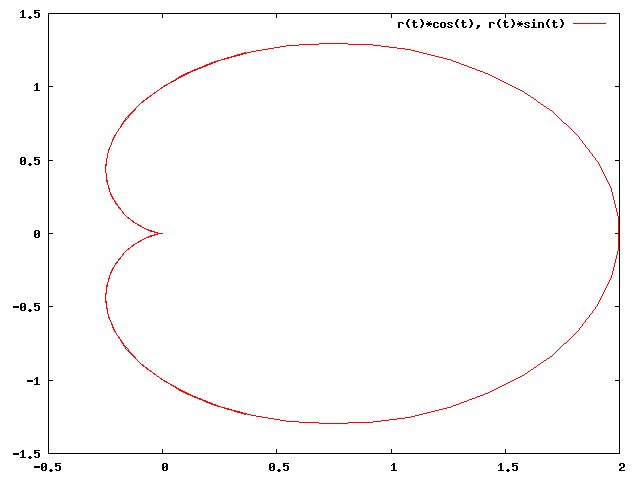
- Cardioid As its name indicates, Cardioid is a heart shaped curve. In spiral's parametric equation, if we put r(t) = 1 + Cos(t) , the result is a cardioid.
gnuplot> set parametric gnuplot> r(t) = 1 + cos(t) gnuplot> plot r(t)cos(t), r(t)sin(t)
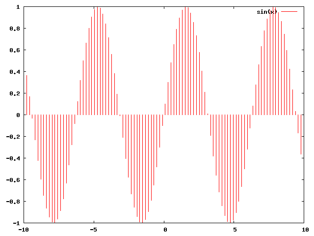
Plotting Styles plot command can take different options like lines, impulses, boxes, points, linespoints etc
gnuplot> plot sin(x) with impulses
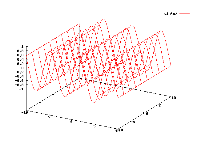
3D Plotting
splot is the command used for 3-dimensional plotting.
gnuplot> splot sin(x)
Click and drag with mouse to rotate the figure 3-dimensionally.
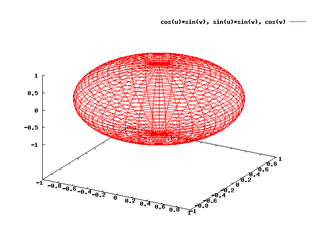
i. Sphere
Parametric equations are:
x = cos(u)sin(v) y = sin(u)sin(v) z = cos(v)
gnuplot> set parametric gnuplot> set urange [0:2pi] gnuplot> set vrange [0:pi] gnuplot> set isosample 40 gnuplot> splot cos(u)sin(v),sin(u)*sin(v),cos(v)
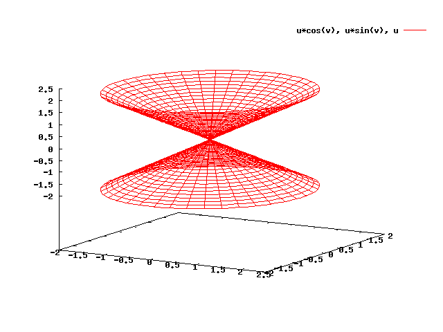
ii. Cone
Parametric equations are:
x = r cos(t) y = r sin(t) z = t
gnuplot> set parametric gnuplot> set urange [-2:2] gnuplot> set vrange [0:2pi] gnuplot> set isosample 40 gnuplot> set view 75,30 gnuplot> splot ucos(v),u*sin(v),u
Parametric equations for 3d figures were obtained from Introduction to gnuplot for Vector Calculus